Visualizing Chicago Public Transit Ridership
In this post, I used Open data from Chicago Transit Authority (CTA) to segment routes based on ridership, and developed a visualization dashboard to identify stops with unbalanced boardings and alightings and stops with the most ridership. Get the raw data here.
load package
library(knitr)
library(tidyverse)
library(stringr)
library(sf)
library(kableExtra)
library(RColorBrewer)
library(viridis)
library(leaflet)
library(ggmap)
library(widgetframe)
raw_df<- read_csv("CTA_-_Ridership_-_Avg._Weekday_Bus_Stop_Boardings_in_October_2012.csv")#clean raw_df
raw_df<-
raw_df %>%
mutate( location= str_replace_all(location, "[()]", "")) %>%
separate(location, c("lat", "lon"), sep = ",") %>%
mutate( lat =as.numeric(lat)) %>%
mutate( lon= as.numeric(lon))Table 1 Routes with most stops
#What is the route with the most stops?
routes <-
  raw_df %>%
  separate_rows(routes) %>%
  group_by(routes) %>%
  summarise(Number_of_stops=n_distinct(stop_id)) %>%
  arrange(desc(Number_of_stops))

kable(routes[1:10, ],  booktabs = T) %>%
kable_styling(bootstrap_options = "striped", full_width = F, position = "left")| routes | Number_of_stops |
|---|---|
| 9 | 273 |
| 49 | 242 |
| 151 | 221 |
| 8 | 220 |
| 3 | 213 |
| 82 | 209 |
| 62 | 206 |
| 79 | 206 |
| N5 | 206 |
| 4 | 202 |
Table 2 Stops with the most routes
#What is the stop with the most routes?
stops <-
  raw_df %>%
  mutate(number_of_routes = str_count(routes, "\\d+")) %>%
  arrange(desc(number_of_routes)) %>%
  select(stop_id,on_street, cross_street, routes, number_of_routes)

kable(stops[1:10, ], booktabs = T) %>%
kable_styling(bootstrap_options = "striped", full_width = F, position = "left")| stop_id | on_street | cross_street | routes | number_of_routes |
|---|---|---|---|---|
| 1106 | MICHIGAN | WASHINGTON | 3,4,19,20,26,60,N66,124,143,145,147,148,151,157 | 14 |
| 73 | MICHIGAN | betw. VAN BUREN & CONGRES | 1,3,4,7,J14,26,X28,126,129,132,143,147,148 | 13 |
| 1103 | MICHIGAN | HUBBARD (WRIGLEY BLDG.) | 2,3,10,26,N66,143,144,145,146,147,148,151,157 | 13 |
| 1120 | MICHIGAN | SOUTH WATER | 3,6,20,26,N66,143,144,145,146,147,148,151,157 | 13 |
| 1122 | MICHIGAN | HUBBARD (TRIBUNE BLDG.) | 2,3,10,26,N66,143,144,145,146,147,148,151,157 | 13 |
| 1100 | MICHIGAN | ERIE | 3,10,26,33,125,143,144,145,146,147,148,151 | 12 |
| 1101 | MICHIGAN | OHIO | 2,3,10,26,143,144,145,146,147,148,151,157 | 12 |
| 1102 | MICHIGAN | ILLINOIS | 2,3,10,26,143,144,145,146,147,148,151,157 | 12 |
| 1105 | MICHIGAN | betw. LAKE & RANDOLPH | 3,4,19,26,N66,124,143,145,147,148,151,157 | 12 |
| 1123 | MICHIGAN | GRAND | 2,3,10,26,143,144,145,146,147,148,151,157 | 12 |
Figure 1 Stop Density Map
#get chicago basemap
chi_bb <- c(left = -87.88430,
            bottom = 41.64416,
            right = -87.52570,
            top = 42.06470)

chicago_stamen <- get_stamenmap(bbox = chi_bb, zoom = 11, maptype = 'toner-lite')

# calculate stop density
df_sp <-
  st_as_sf(raw_df, coords = c("lon", "lat"), crs = 4326) %>%
  select(-c('month_beginning','daytype'))

#plot them together
stops_density_map <-
  ggmap(chicago_stamen)+
  stat_density_2d(data = raw_df,
                  aes(x = lon, y = lat, fill = stat(level)),
                  alpha = .4,
                  bins = 5,
                  geom = "polygon") +
  scale_fill_gradientn('number of stops',colors = brewer.pal(5, "YlOrRd")) +
  geom_sf(data = df_sp, inherit.aes = FALSE,color='black',
          size = 0.2, alpha=0.1,show.legend = 'point')

stops_density_map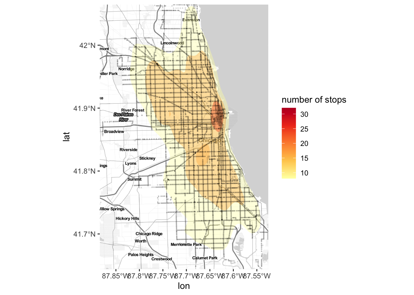
Figure 2 Map of stops with no ridership
#tranform to long dataframe
stops_route <-
  raw_df %>%
  mutate(number_of_routes = str_count(routes, "\\d+")) %>%
  separate_rows(routes) %>%
  mutate( boardings = boardings/number_of_routes) %>%
  mutate(alightings =  alightings/ number_of_routes)  %>%
  select( -c(number_of_routes,daytype,month_beginning)) %>%
  gather("boardings", "alightings", key = type, value = ridership)

#make it sf object
stops_route_sp <-
  st_as_sf(stops_route, coords = c("lon", "lat"), crs = 4326)

#stops with no boardings and alightings
#transform stops_no_ridership to spatial dataframe

stops_no_ridership_sp <-
  stops_route_sp %>%
  filter (ridership==0) %>%
  group_by(stop_id, routes) %>%
  filter(n()>1)

#n_distinct(stops_no_ridership_sp$stop_id)
#n_distinct(stops_no_ridership_sp$routes)

#set color scheme
pal <- colorFactor(palette = 'Spectral', domain =stops_no_ridership_sp$routes)

#plot
p1<-leaflet(stops_no_ridership_sp) %>%
  setView(lng=-87.705, lat=41.85443, zoom = 10) %>%
  addProviderTiles(providers$Stamen.Toner,group="Stamen Toner") %>%
  addCircleMarkers( color = ~pal(routes),
                        radius = ~ ifelse(ridership <=100, 6,
                                           ifelse((ridership <=1000),10,15)),
                        stroke = FALSE,
                        fillOpacity = 0.8,
                        popup = ~paste("Stop_id:", stop_id,
                          "<br>", "Route:", routes,
                          "<br>", "Ridership:", ridership)) %>%
      addLegend("topright", pal = pal, opacity = 1,
                values = ~routes,
                title = "Routes")
frameWidget(p1, width='100%')
Table 3 Top 10 most trafficked routes
#routes by boarding and alighting ridership
ridership_by_routes<-
  stops_route %>%
  filter(!is.na(routes)) %>%
  group_by(routes, type) %>%
  summarise(n=sum(ridership)) %>%
  spread(type, n) %>%
  mutate(total =boardings+ alightings) %>%
  arrange(desc(total))

kable(ridership_by_routes[1:10, ], booktabs = T) %>%
kable_styling(bootstrap_options = "striped", full_width = F, position = "left")| routes | alightings | boardings | total |
|---|---|---|---|
| 9 | 33119.68 | 33704.75 | 66824.43 |
| 79 | 31520.93 | 31741.53 | 63262.47 |
| 49 | 29305.87 | 29500.68 | 58806.55 |
| 66 | 26494.62 | 26566.83 | 53061.45 |
| 77 | 24193.93 | 22996.52 | 47190.45 |
| 8 | 23579.65 | 23555.37 | 47135.02 |
| 53 | 23540.77 | 23586.90 | 47127.67 |
| 4 | 23855.90 | 22107.08 | 45962.98 |
| 82 | 22379.65 | 22005.20 | 44384.85 |
| 63 | 21785.53 | 21732.61 | 43518.14 |
Figure 3 Stops segmentation based on Ridership
#reshape df with only lat, lon, boardings, and alights columns
#scale the dataset
km_df_scale<-
  raw_df%>%
  select(stop_id,boardings,alightings) %>%
  column_to_rownames(var="stop_id") %>%
  scale()
library(factoextra)
set.seed(123)
# function to compute total within-cluster sum of square
wss <- function(k) {
kmeans(km_df_scale, k,iter.max = 100, nstart = 25 )$tot.withinss
}
# Compute and plot wss for k = 1 to k = 15
k.values <- 1:15
# extract wss for 2-15 clusters
wss_values <- map_dbl(k.values, wss)
#plot optimal K
plot(k.values, wss_values,
type="b", pch = 19, frame = FALSE,
xlab="Number of clusters K",
ylab="Total within-clusters sum of squares")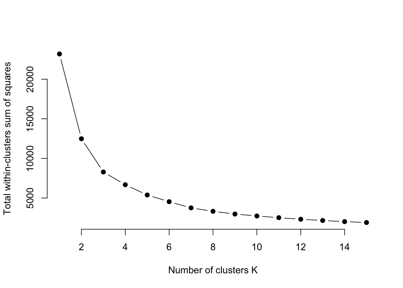
set.seed(123)

#kmeans with 3 clusters
km.res <- kmeans(km_df_scale, 3, iter.max = 100, nstart = 25)

#join with raw df
dd <- cbind(raw_df, cluster = km.res$cluster)

#plot
dd %>%
  ggplot(aes(x=boardings, y= alightings, color= factor(cluster))) +
  geom_point() +
  geom_abline(aes(intercept = 0 , slope= 1 ), linetype= "dashed") +
  scale_x_continuous(trans = 'log') +
  scale_y_continuous(trans = 'log') +
  scale_size(range = c(0.5, 5))  +
  scale_color_brewer("", palette = "Set1",
                     labels = c("Stops with little ridership",
                                "Stops with most ridership",
                                "Stops with medium ridership")) +
  theme_bw() +
  xlab("Boardings") +
ylab("Alightings") 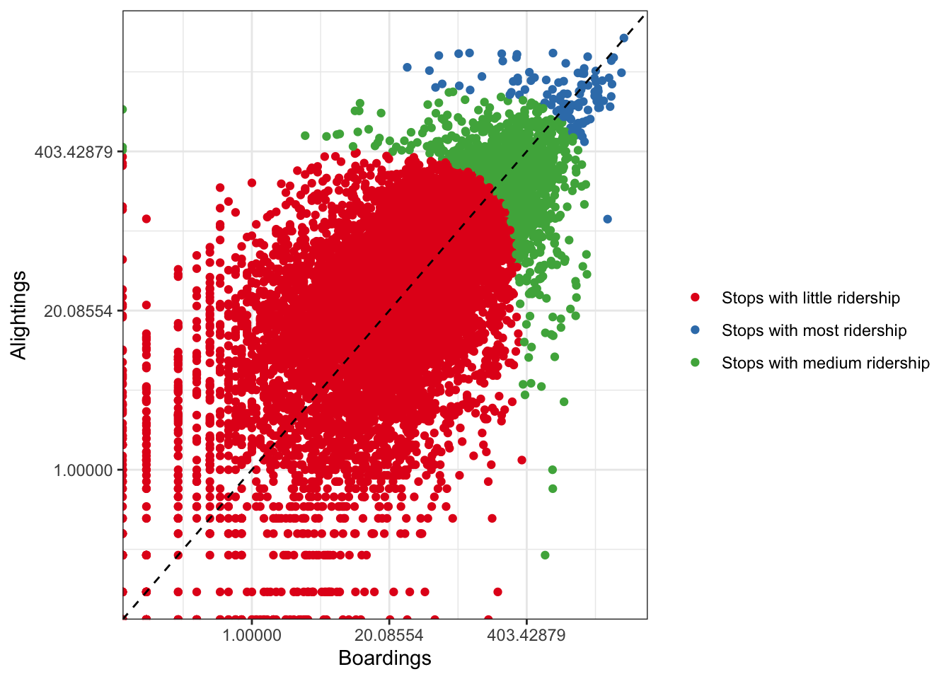
#visualize on a map
m = leaflet() %>%
    setView(lng=-87.705, lat=41.85443, zoom = 10) %>%
    addProviderTiles(providers$Stamen.Toner,group="Stamen Toner")

# subset into clusters
data_filterlist = list(cluster_1 = subset(dd, cluster == 1),
                cluster_2 = subset(dd, cluster == 2),
                cluster_3 = subset(dd, cluster == 3))

# Remember we also had these groups associated with each variable? Let's put them in a list too:
layerlist = c("Stops with little ridership", "Stops with most ridership", "Stops with medium ridership")

# We can keep that same color variable:
colorFactors = colorFactor(c('red', 'blue', 'seagreen'), domain=dd$cluster)

# Now we have our loop - each time through the loop, it is adding our markers to the map object:

for (i in 1:length(data_filterlist)){
  m = addCircleMarkers(m,
                       lng=data_filterlist[[i]]$lon,
                       lat=data_filterlist[[i]]$lat,
                       radius=1,
                       popup= paste( "Stop_id:",data_filterlist[[i]]$stop_id,
                                     "<br>", "Routes:", data_filterlist[[i]]$routes,
                                     "<br>", "Boardings:",data_filterlist[[i]]$boardings,
                                     "<br>", "Alightings:",data_filterlist[[i]]$alightings),
                       stroke = FALSE, fillOpacity = 0.75,
                       color = colorFactors(data_filterlist[[i]]$cluster),
                       group = layerlist[i]
  )

}


p2<- addLayersControl(m, overlayGroups = layerlist, options = layersControlOptions(collapsed = FALSE))

frameWidget(p2, width='100%')